Drug Repurposing from Transcriptomic Data

Introduction

Drug repurposing (also called drug repositioning) is the process of identifying new therapeutic uses for existing drugs. This approach offers several advantages over traditional drug discovery:

Reduced development time: Existing drugs have known safety profiles
Lower costs: Skip early-stage development and toxicity testing
Higher success rates: Known pharmacokinetics and pharmacodynamics
Rapid clinical translation: Faster path to patient benefit

This vignette demonstrates how to use drugfindR to identify candidate repurposable drugs from transcriptomic signatures of disease states.

Prerequisites

library(drugfindR)
library(dplyr)
library(readr)
library(ggplot2)
library(tidyr)

The Drug Repurposing Workflow

The typical workflow involves:

Obtain disease signature: Differential expression analysis from disease vs. control
Prepare signature: Format for iLINCS compatibility
Filter genes: Select most differentially expressed genes
Query iLINCS: Find drugs with opposing signatures (anti-correlated)
Rank candidates: Prioritize based on similarity scores
Validate: Literature review, experimental validation

Case Study: COVID-19 Drug Repurposing

We’ll use a published COVID-19 transcriptomic signature to demonstrate the workflow. This example replicates aspects of the analysis from O’Donovan et al. (2021).

Step 1: Load Disease Signature

# Load pre-computed differential expression results
covid_file <- system.file("extdata", "dCovid_diffexp.tsv", package = "drugfindR")
covid_diffexp <- read_tsv(covid_file, show_col_types = FALSE)

# Examine the data structure
cat("Dimensions:", nrow(covid_diffexp), "genes x", ncol(covid_diffexp), "columns\n")
#> Dimensions: 4090 genes x 3 columns
head(covid_diffexp)
#> # A tibble: 6 × 3
#>   hgnc_symbol logFC     PValue
#>   <chr>       <dbl>      <dbl>
#> 1 CCL4L2      -3.98 0.00000177
#> 2 IL5RA       -4.83 0.00000870
#> 3 FN1          4.94 0.0000117 
#> 4 GSTM1       -8.21 0.0000153 
#> 5 CD180        2.15 0.0000202 
#> 6 FAM20C       3.11 0.0000255

This dataset contains differential expression results from SARS-CoV-2 infected cells:

hgnc_symbol: HGNC gene symbols
logFC: Log2 fold-change (infected vs. control)
PValue: Statistical significance

# Summary statistics
cat(
    "Log fold-change range:",
    round(min(covid_diffexp$logFC), 2), "to",
    round(max(covid_diffexp$logFC), 2), "\n"
)
#> Log fold-change range: -8.76 to 9.95
cat(
    "Significant genes (p < 0.01):",
    sum(covid_diffexp$PValue < 0.01), "\n"
)
#> Significant genes (p < 0.01): 1044

Step 2: Visualize the Signature

Understanding your signature helps inform filtering decisions.

# Volcano plot
ggplot(covid_diffexp, aes(x = logFC, y = -log10(PValue))) +
    geom_point(aes(color = abs(logFC) > 1.5 & PValue < 0.01),
        alpha = 0.6, size = 1.5
    ) +
    scale_color_manual(
        values = c("gray70", "red3"),
        labels = c("Not significant", "Significant"),
        name = ""
    ) +
    geom_vline(xintercept = c(-1.5, 1.5), linetype = "dashed", color = "blue") +
    geom_hline(yintercept = -log10(0.01), linetype = "dashed", color = "blue") +
    labs(
        title = "COVID-19 Infection Signature Volcano Plot",
        x = "Log2 Fold Change",
        y = "-Log10(P-value)"
    ) +
    theme_minimal() +
    theme(legend.position = "bottom")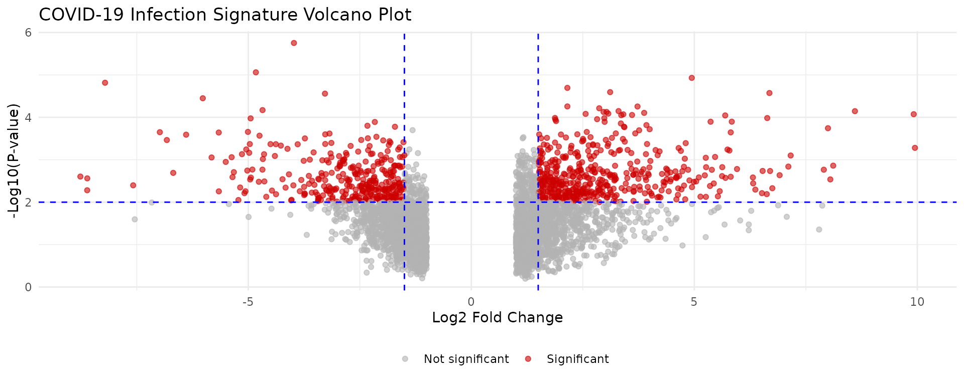

# Distribution of log fold-changes
ggplot(covid_diffexp, aes(x = logFC)) +
    geom_histogram(bins = 50, fill = "steelblue", alpha = 0.7) +
    geom_vline(xintercept = c(-1.5, 1.5), linetype = "dashed", color = "red") +
    labs(
        title = "Distribution of Log Fold-Changes",
        x = "Log2 Fold Change",
        y = "Number of Genes"
    ) +
    theme_minimal()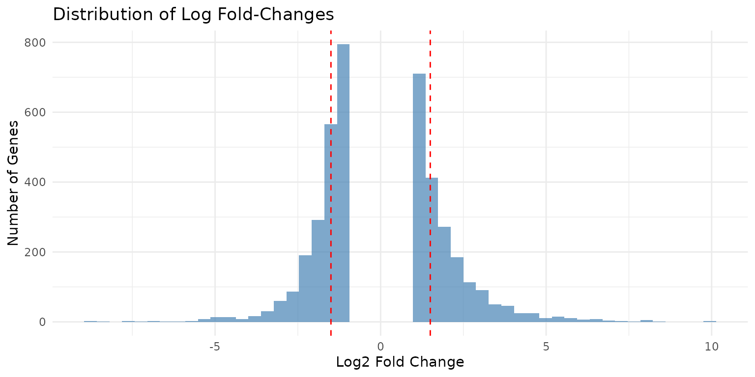

Step 3: Choose Filtering Strategy

Strategy A: Absolute Threshold

Select genes with large magnitude changes:

# Prepare signature for iLINCS
signature <- prepareSignature(
    covid_diffexp,
    geneColumn = "hgnc_symbol",
    logfcColumn = "logFC",
    pvalColumn = "PValue"
)

cat("Signature prepared with", nrow(signature), "L1000 genes\n")
#> Signature prepared with 170 L1000 genes

# Filter with symmetric threshold
filtered_threshold <- filterSignature(signature, threshold = 1.5)
cat("Genes with |logFC| >= 1.5:", nrow(filtered_threshold), "\n")
#> Genes with |logFC| >= 1.5: 87

# Separate by direction
up_genes <- filterSignature(signature, direction = "up", threshold = 1.5)
down_genes <- filterSignature(signature, direction = "down", threshold = 1.5)

cat("Upregulated (>= 1.5):", nrow(up_genes), "\n")
#> Upregulated (>= 1.5): 72
cat("Downregulated (<= -1.5):", nrow(down_genes), "\n")
#> Downregulated (<= -1.5): 15

Strategy B: Proportional Threshold

Select a fixed percentage of most extreme genes:

# Top and bottom 5% most differentially expressed
filtered_prop <- filterSignature(signature, prop = 0.05)
cat("Top/bottom 5%:", nrow(filtered_prop), "genes\n")
#> Top/bottom 5%: 18 genes

# Compare strategies
cat("\nComparing strategies:\n")
#> 
#> Comparing strategies:
cat("Absolute threshold (1.5):", nrow(filtered_threshold), "genes\n")
#> Absolute threshold (1.5): 87 genes
cat("Proportional (5%):", nrow(filtered_prop), "genes\n")
#> Proportional (5%): 18 genes

Strategy C: Asymmetric Threshold

Different thresholds for up and down regulation:

# More stringent for upregulation
filtered_asym <- filterSignature(signature, threshold = c(-1.0, 2.0))
cat(
    "Asymmetric filtering (down <= -1.0, up >= 2.0):",
    nrow(filtered_asym), "genes\n"
)
#> Asymmetric filtering (down <= -1.0, up >= 2.0): 73 genes

Step 4: Query iLINCS for Concordant Drugs

# Query Chemical Perturbagen library
concordants_up <- getConcordants(
    up_genes,
    ilincsLibrary = "CP",
    direction = "up"
)

concordants_down <- getConcordants(
    down_genes,
    ilincsLibrary = "CP",
    direction = "down"
)

cat("Concordant signatures found:\n")
cat("  Up-regulated matches:", nrow(concordants_up), "\n")
cat("  Down-regulated matches:", nrow(concordants_down), "\n")

Step 5: Generate Consensus Rankings

# Combine and rank candidates
consensus <- consensusConcordants(
    concordants_up,
    concordants_down,
    paired = TRUE,
    cutoff = 0.2 # Minimum absolute similarity
)

# Preview results
head(consensus, 15)

Step 6: One-Step Convenience Function

For standard workflows, use the convenience function:

# Complete analysis in one call
drug_candidates <- investigateSignature(
    expr = covid_diffexp,
    outputLib = "CP",
    filterThreshold = 1.5,
    similarityThreshold = 0.2,
    paired = TRUE,
    geneColumn = "hgnc_symbol",
    logfcColumn = "logFC",
    pvalColumn = "PValue",
    sourceName = "COVID19_Infection",
    sourceCellLine = "HumanLungCells"
)

# View top candidates
head(drug_candidates, 20)

Interpreting Results

Understanding Similarity Scores

The similarity score indicates concordance between signatures:

-1.0 to -0.3: Strong opposition (drug reverses disease signature) ⭐
-0.3 to 0: Weak opposition
0 to 0.3: Weak agreement
0.3 to 1.0: Strong agreement (drug mimics disease)

For drug repurposing, we want negative similarity scores (anti-correlated).

Filtering Candidate Results

# Identify top therapeutic candidates
therapeutic_candidates <- drug_candidates %>%
    filter(Similarity < -0.3) %>% # Strong opposition
    arrange(Similarity) %>% # Most opposing first
    distinct(Target, .keep_all = TRUE) # Unique drugs

# View top 10 candidates
head(therapeutic_candidates, 10)

Considering Statistical Significance

# Filter by both similarity and significance
high_confidence <- drug_candidates %>%
    filter(Similarity < -0.3, pValue < 0.05) %>%
    arrange(Similarity)

cat("High-confidence candidates:", nrow(high_confidence), "\n")

Cell Line-Specific Analysis

Different cell lines may respond differently to treatments.

Restricting to Relevant Cell Lines

# For lung disease, focus on lung-derived cell lines
lung_candidates <- investigateSignature(
    expr = covid_diffexp,
    outputLib = "CP",
    filterThreshold = 1.5,
    outputCellLines = c("A549", "HBEC3KT", "NCI-H1299"),
    geneColumn = "hgnc_symbol",
    logfcColumn = "logFC",
    pvalColumn = "PValue"
)

Analyzing Cross-Cell Line Consistency

# Get results without cell line restriction
all_celllines <- investigateSignature(
    expr = covid_diffexp,
    outputLib = "CP",
    filterThreshold = 1.5,
    geneColumn = "hgnc_symbol",
    logfcColumn = "logFC",
    pvalColumn = "PValue"
)

# Identify drugs active across multiple cell lines
multi_cellline <- all_celllines %>%
    group_by(Target) %>%
    summarize(
        n_celllines = n_distinct(TargetCellLine),
        mean_similarity = mean(Similarity),
        .groups = "drop"
    ) %>%
    filter(n_celllines >= 3, mean_similarity < -0.3) %>%
    arrange(mean_similarity)

head(multi_cellline, 10)

Comparing Paired vs. Unpaired Analysis

Paired Analysis

Treats up- and down-regulated genes separately:

results_paired <- investigateSignature(
    expr = covid_diffexp,
    outputLib = "CP",
    filterThreshold = 1.5,
    paired = TRUE, # Separate up/down analysis
    geneColumn = "hgnc_symbol",
    logfcColumn = "logFC",
    pvalColumn = "PValue"
)

Advantages: - Captures directional biology - More precise matching - Better for asymmetric signatures

Unpaired Analysis

Treats all significant genes together:

results_unpaired <- investigateSignature(
    expr = covid_diffexp,
    outputLib = "CP",
    filterThreshold = 1.5,
    paired = FALSE, # Combined analysis
    geneColumn = "hgnc_symbol",
    logfcColumn = "logFC",
    pvalColumn = "PValue"
)

Advantages: - Simpler interpretation - Faster execution - Good for symmetric signatures

Comparing Results

# Compare number of candidates
cat("Paired analysis candidates:", nrow(results_paired), "\n")
cat("Unpaired analysis candidates:", nrow(results_unpaired), "\n")

# Find overlap in top candidates
top_paired <- results_paired %>%
    filter(Similarity < -0.3) %>%
    pull(Target)

top_unpaired <- results_unpaired %>%
    filter(Similarity < -0.3) %>%
    pull(Target)

overlap <- intersect(top_paired, top_unpaired)
cat("Overlap in top candidates:", length(overlap), "\n")

Visualization of Results

Top Candidates Bar Plot

top_20 <- drug_candidates %>%
    filter(Similarity < 0) %>%
    arrange(Similarity) %>%
    head(20)

ggplot(top_20, aes(x = reorder(Target, Similarity), y = Similarity)) +
    geom_col(aes(fill = Similarity < -0.3), show.legend = FALSE) +
    scale_fill_manual(values = c("steelblue", "red3")) +
    coord_flip() +
    labs(
        title = "Top 20 Drug Candidates for COVID-19",
        x = "Drug/Compound",
        y = "Similarity Score (more negative = better)"
    ) +
    theme_minimal() +
    theme(axis.text.y = element_text(size = 10))

Similarity Distribution

ggplot(drug_candidates, aes(x = Similarity)) +
    geom_histogram(bins = 50, fill = "steelblue", alpha = 0.7) +
    geom_vline(xintercept = -0.3, linetype = "dashed", color = "red", size = 1) +
    geom_vline(xintercept = 0, linetype = "solid", color = "black") +
    labs(
        title = "Distribution of Drug Similarity Scores",
        x = "Similarity Score",
        y = "Number of Drug Signatures",
        subtitle = "Red line: therapeutic threshold (-0.3)"
    ) +
    theme_minimal()

Cell Line Heatmap

# Prepare data for heatmap
heatmap_data <- drug_candidates %>%
    filter(Similarity < -0.2) %>%
    group_by(Target) %>%
    filter(n() >= 2) %>% # Drugs tested in multiple cell lines
    ungroup() %>%
    select(Target, TargetCellLine, Similarity) %>%
    head(50) # Top candidates

ggplot(heatmap_data, aes(x = TargetCellLine, y = Target, fill = Similarity)) +
    geom_tile(color = "white") +
    scale_fill_gradient2(
        low = "blue", mid = "white", high = "red",
        midpoint = 0,
        name = "Similarity"
    ) +
    labs(
        title = "Drug Activity Across Cell Lines",
        x = "Cell Line",
        y = "Drug"
    ) +
    theme_minimal() +
    theme(
        axis.text.x = element_text(angle = 45, hjust = 1),
        axis.text.y = element_text(size = 8)
    )

Working with DESeq2 Output

Integration with standard Bioconductor workflows:

# Assume you have DESeq2 results
# library(DESeq2)
# dds <- DESeq(dds)
# res <- results(dds)

# Convert DESeq2 results to data frame
# deseq2_results <- as.data.frame(res) %>%
#     tibble::rownames_to_column("gene") %>%
#     filter(!is.na(padj))

# Use with drugfindR
# drug_candidates <- investigateSignature(
#     expr = deseq2_results,
#     outputLib = "CP",
#     filterThreshold = 1.5,
#     geneColumn = "gene",
#     logfcColumn = "log2FoldChange",
#     pvalColumn = "pvalue"
# )

Working with edgeR Output

# Assume you have edgeR results
# library(edgeR)
# et <- exactTest(dge)
# edger_results <- topTags(et, n = Inf)$table

# Convert to appropriate format
# edger_df <- edger_results %>%
#     tibble::rownames_to_column("gene")

# Use with drugfindR
# drug_candidates <- investigateSignature(
#     expr = edger_df,
#     outputLib = "CP",
#     filterThreshold = 1.5,
#     geneColumn = "gene",
#     logfcColumn = "logFC",
#     pvalColumn = "PValue"
# )

Best Practices

1. Threshold Selection

Conservative (1.5-2.0): High confidence, fewer genes
Moderate (1.0-1.5): Balanced approach (recommended starting point)
Liberal (0.5-1.0): Broader coverage, more candidates
Proportional (5-10%): Data-adaptive approach

2. Quality Control

# Check for adequate differential expression
sig_genes <- sum(abs(covid_diffexp$logFC) > 1.0)
if (sig_genes < 50) {
    warning("Few significantly DE genes. Consider lowering threshold.")
}

# Verify L1000 gene coverage
l1000_coverage <- nrow(signature) / nrow(covid_diffexp) * 100
cat("L1000 gene coverage:", round(l1000_coverage, 1), "%\n")

3. Validation Strategy

After computational screening:

Literature validation: Check PubMed for prior evidence
Mechanism review: Understand drug’s known mechanisms
Safety assessment: Review known side effects
Dose consideration: Consider therapeutic dose ranges
Experimental validation: In vitro/in vivo testing

4. Multiple Hypothesis Testing

# Adjust p-values for multiple comparisons
drug_candidates_adjusted <- drug_candidates %>%
    mutate(pValue_adjusted = p.adjust(pValue, method = "BH"))

# Filter with adjusted p-values
validated_candidates <- drug_candidates_adjusted %>%
    filter(Similarity < -0.3, pValue_adjusted < 0.05)

Advanced Filtering Scenarios

Scenario 1: Highly Specific Signature

Few but very strong changes:

specific_results <- investigateSignature(
    expr = covid_diffexp,
    outputLib = "CP",
    filterThreshold = 2.5, # Very stringent
    similarityThreshold = 0.3, # Higher similarity required
    paired = TRUE,
    geneColumn = "hgnc_symbol",
    logfcColumn = "logFC",
    pvalColumn = "PValue"
)

Scenario 2: Broad Signature

Many moderate changes:

broad_results <- investigateSignature(
    expr = covid_diffexp,
    outputLib = "CP",
    filterProp = 0.15, # Top/bottom 15%
    similarityThreshold = 0.15, # Lower threshold
    paired = TRUE,
    geneColumn = "hgnc_symbol",
    logfcColumn = "logFC",
    pvalColumn = "PValue"
)

Scenario 3: Direction-Specific Interest

Only interested in downregulated genes:

# Manual approach for maximum control
sig_prepared <- prepareSignature(covid_diffexp, geneColumn = "hgnc_symbol")
down_only <- filterSignature(sig_prepared, direction = "down", threshold = 1.5)
down_concordants <- getConcordants(down_only, ilincsLibrary = "CP")
down_consensus <- consensusConcordants(down_concordants, paired = FALSE, cutoff = 0.2)

Troubleshooting

Empty Results

If you get no results:

# 1. Lower filtering threshold
relaxed_results <- investigateSignature(
    expr = covid_diffexp,
    outputLib = "CP",
    filterThreshold = 0.5, # Lower threshold
    geneColumn = "hgnc_symbol"
)

# 2. Use proportional filtering
prop_results <- investigateSignature(
    expr = covid_diffexp,
    outputLib = "CP",
    filterProp = 0.2, # Top 20%
    geneColumn = "hgnc_symbol"
)

# 3. Lower similarity threshold
liberal_results <- investigateSignature(
    expr = covid_diffexp,
    outputLib = "CP",
    filterThreshold = 1.0,
    similarityThreshold = 0.1, # Very permissive
    geneColumn = "hgnc_symbol"
)

Too Many Results

If results are overwhelming:

# Increase thresholds
stringent_results <- investigateSignature(
    expr = covid_diffexp,
    outputLib = "CP",
    filterThreshold = 2.0, # More stringent
    similarityThreshold = 0.3, # Higher cutoff
    geneColumn = "hgnc_symbol"
)

# Focus on specific cell lines
focused_results <- investigateSignature(
    expr = covid_diffexp,
    outputLib = "CP",
    filterThreshold = 1.5,
    outputCellLines = c("A549", "MCF7", "PC3"),
    geneColumn = "hgnc_symbol"
)

Summary

Key takeaways for drug repurposing with drugfindR:

Start with quality DE data: Strong differential expression signal
Choose appropriate thresholds: Balance sensitivity and specificity
Use paired analysis: For complex, asymmetric signatures
Look for negative similarity: Anti-correlated drugs are therapeutic candidates
Consider cell line context: Tissue-relevant models
Validate computationally: Literature, mechanisms, safety
Plan experimental validation: Essential for translation

Next Steps

Target Investigation: Explore gene-drug relationships
Getting Started: Quick start guide
Function Reference: Complete API documentation

Session Information

sessionInfo()
#> R version 4.6.1 (2026-06-24)
#> Platform: x86_64-pc-linux-gnu
#> Running under: Ubuntu 24.04.4 LTS
#> 
#> Matrix products: default
#> BLAS:   /usr/lib/x86_64-linux-gnu/openblas-pthread/libblas.so.3 
#> LAPACK: /usr/lib/x86_64-linux-gnu/openblas-pthread/libopenblasp-r0.3.26.so;  LAPACK version 3.12.0
#> 
#> locale:
#>  [1] LC_CTYPE=C.UTF-8       LC_NUMERIC=C           LC_TIME=C.UTF-8       
#>  [4] LC_COLLATE=C.UTF-8     LC_MONETARY=C.UTF-8    LC_MESSAGES=C.UTF-8   
#>  [7] LC_PAPER=C.UTF-8       LC_NAME=C              LC_ADDRESS=C          
#> [10] LC_TELEPHONE=C         LC_MEASUREMENT=C.UTF-8 LC_IDENTIFICATION=C   
#> 
#> time zone: UTC
#> tzcode source: system (glibc)
#> 
#> attached base packages:
#> [1] stats     graphics  grDevices utils     datasets  methods   base     
#> 
#> other attached packages:
#> [1] tidyr_1.3.2      ggplot2_4.0.3    readr_2.2.0      dplyr_1.2.1     
#> [5] drugfindR_1.0.0  BiocStyle_2.40.0
#> 
#> loaded via a namespace (and not attached):
#>  [1] utf8_1.2.6          rappdirs_0.3.4      sass_0.4.10        
#>  [4] generics_0.1.4      stringi_1.8.7       hms_1.1.4          
#>  [7] digest_0.6.39       magrittr_2.0.5      RColorBrewer_1.1-3 
#> [10] evaluate_1.0.5      grid_4.6.1          bookdown_0.47      
#> [13] fastmap_1.2.0       jsonlite_2.0.0      DFplyr_1.6.0       
#> [16] BiocManager_1.30.27 purrr_1.2.2         scales_1.4.0       
#> [19] httr2_1.2.3         textshaping_1.0.5   jquerylib_0.1.4    
#> [22] cli_3.6.6           crayon_1.5.3        rlang_1.3.0        
#> [25] bit64_4.8.2         withr_3.0.3         cachem_1.1.0       
#> [28] yaml_2.3.12         otel_0.2.0          parallel_4.6.1     
#> [31] tools_4.6.1         tzdb_0.5.0          BiocGenerics_0.58.1
#> [34] curl_7.1.0          vctrs_0.7.3         R6_2.6.1           
#> [37] stats4_4.6.1        lifecycle_1.0.5     stringr_1.6.0      
#> [40] bit_4.6.0           S4Vectors_0.50.1    fs_2.1.0           
#> [43] htmlwidgets_1.6.4   vroom_1.7.1         ragg_1.5.2         
#> [46] pkgconfig_2.0.3     desc_1.4.3          pkgdown_2.2.1      
#> [49] pillar_1.11.1       bslib_0.11.0        gtable_0.3.6       
#> [52] glue_1.8.1          systemfonts_1.3.2   xfun_0.60          
#> [55] tibble_3.3.1        tidyselect_1.2.1    knitr_1.51         
#> [58] farver_2.1.2        htmltools_0.5.9     labeling_0.4.3     
#> [61] rmarkdown_2.31      compiler_4.6.1      S7_0.2.2

References

O’Donovan SM, Imami A, et al. (2021). Identification of candidate repurposable drugs to combat COVID-19 using a signature-based approach. Scientific Reports, 11:4495.
Pushpakom S, et al. (2019). Drug repurposing: progress, challenges and recommendations. Nature Reviews Drug Discovery, 18:41-58.
Subramanian A, et al. (2017). A Next Generation Connectivity Map: L1000 Platform and the First 1,000,000 Profiles. Cell, 171(6):1437-1452.

Ali Sajid Imami

2026-07-10